One of my recent projects involved running our flagship carbon model at a 1km (0.0083°) resolution. Models like these are usually run at ~50km (0.5°), so this represents a significant scale up - a 3600x1 increase in resolution and three orders of magnitude more simulations. Accomplishing this took model optimizations in C, HPC engineering, tens of TBs of storage and ~50 CPU years of compute. The scale of the problem exposed weaknesses in our infrastructure whose solutions will keep accelerating our analyses into the future.
The results, driven by the CHELSA meteorology dataset, align well with other estimates of key ecological variables. There are a ton of research opportunities that this enables. For example, we’re involved in an effort to assess the value-add of using high resolution data in the climate/ecological model space, which will be done sometime in the fall. Stay tuned!
See below for a small sample on CONUS (use the slider to compare images, and make sure to zoom in!):
Conterminous U.S. GPP for June 2016. High res (left) is CHELSA driven LPJ, low res (right) is ERA5 driven. 0 values are set to NaN. Spatial differences are due to the differences in the input drivers. CONUS-only because the filesizes are small enough for GH and I don't want to host on S3 and incur egress costs.
A short description of the problem, the solution, and some takeaways
LPJ-Earth Observation SIMulator (LPJ-EOSIM)
LPJ-EOSIM is complex, requiring thousands of calibration steps before being able to model real-world quantities accurately. Once it’s properly “spun-up”, it can be used to estimate some important quantities, like how much CO2 is absorbed by land vegetation every year2. LPJ has been around for ~25 years and historically has been run at a 0.5° (~50km) resolution, mostly for computational and input data resolution issues.
I/O refactoring, chunking, and GPFS
When I started at NASA, LPJ could only run with monthly datasets as input and even this took ~24 hours. LPJ’s I/O scheme combined with GPFS didn’t work with daily datasets. Using it on a 1km daily dataset would’ve been impossible and wasn’t on the horizon.
I refactored the I/O module in LPJ to play a little more nicely with GPFS and rechunked the input netCDFs to align with our loading strategy. These modifications meant a global run3 now completed in ~20 minutes and was CPU-bound4. The model was sped up ~100x on monthly datasets and went from being unusable with daily datasets to being fast.
With these optimizations in hand running on a global 1km dataset was possible. At this point, the engineering switched from C development to workflow orchestration on Discover5.
Some back of the envelope calculations6 had the number of simulations in the thousands. The scope of this was far greater than any number of simulations that we needed to run before - we’d do maybe 20 or so simulations at a time on a few different driver sets.
LPJ parallelization and splitting the CHELSA meteorology
We run a process-level embarrassingly parallel workflow with LPJ, where each process processes a distinct set of coordinates from the input dataset and writes a set of output diagnostics. The CHELSA meteorology dataset is roughly 40k$\times$20k cells, and a good rule of thumb for number of cells per core is ~500. Reading 500 cells per process from a single 40k$\times$20k raster with hundreds of processes is a good recipe for getting yourself kicked off the cluster. GPFS doesn’t thrive when many processes do I/O on the same directory, not to mention the same file in that directory.
I wrote a simple algorithm to iteratively grow slices of latitude into rectangles containing at most 200k cells, the results of which are shown in the figure below. Each chunk was then loaded into LPJ separately.
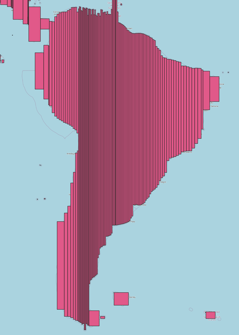 The grid split algorithm on South America.
Why 200k? On a shared-resource cluster you want jobs that will run in a reasonable amount of time (1-4 hours) so they clear the queue quickly, but you don’t want to request so many resources that a single job’s allocation sits in the queue for a long time. In addition, each LPJ process emits something like 35 files, so I needed to keep the number of CPUs per job small to reduce file load on the cluster since we’re subject to hard limits.
Once the splits were extracted from the global CHELSA rasters, I spun up dask clusters so I could apply arbitrary python logic to
format the drivers for each split correctly. I designed the drivers to be ephemeral because persisting them on disk would’ve been too expensive.
Updating the parallelization pipeline
The pipeline for distributing LPJ across computing ecosystems evolved over many years and many supercomputers and was originally in bash.
I replicated the set of bash scripts in python, and kept most of the core simulation logic (distribution strategy, job queueing, etc).
The core simulation logic wasn’t robust enough to handle the CHELSA dataset. Also, running something at thousands of times its intended usage will inevitably expose bottlenecks.
I added around ~10 necessary optimizations to the pipeline which allowed simulations to work through the queue quickly, which included using dask, refactoring the SLURM interaction,
and auto-tarring simulation output.
Blockers, non-technical lessons learned
- I was under a time crunch to get these simulations done, so I wrote some hacky code at times that was immediate tech debt. This is a reminder to slow down and follow DRY.
- I didn’t test the algorithm for creating a global grid split and an edge case slipped by, leading to some re-runs. Note to self: tests for that sort of code are pretty important. Again, though, with a time crunch it’s tough.
- I should’ve questioned the assumptions of the old pipeline sooner.
- Misinterpretation of LPJ’s internals meant I had to re-do part of the analysis - get a second pair of eyes on things!
Next steps
Use prefect and dask to make the pipeline truly production grade. dask was a force multiplier during this process. Parallelizing Python on SLURM is a huge workflow enhancement.
It’s sort of hard to come up with meaningful example of what it means to scale up something by 3600x. $log_2(3600)\approx12$, so we could cast it as 12 cycles of Moore’s law, or ~24 years of semiconductor development. Imagine what your desktop could do in 2000 and compare that to now. For us, though, it means way better diagnostics. ↩︎
This is important for a variety of reasons, including estimating the buffer the land provides against anthropogenic CO2 emissions. However, this is not the main point of this article. For an overview of what models like LPJ-EOSIM can do, see the Global Carbon Project’s Global Carbon Budget. ↩︎
This is for a simple simulation protocol at a level of parallelization enabled by the aforementioned I/O refactoring and input chunking. ↩︎
-O3means it screams. Probably could speed the model up more by more simple optimizations and SIMD, but sometimes the lowest hanging fruits are the only ones you need to pick. ↩︎Discover is a supercomputer at NASA Goddard that has made the Top500 list. ↩︎
0.5°: 720x360 cells = 259200 total cells, 67420 of which are land surface. 1km: 40k by 20k cells, multiplied by (67420/259200) ~ $200\times10^6$. ↩︎